A little while ago I showed Karthik Ram the percent function from scales, and he said something along the lines of:
There should be a high quality screencase where someone shows a couple of rstats tricks and thats it.
So this is it! I just uploaded a screencast to youtube called “Just Three Things”. I can’t promise that it is as high quality as I would have liked, but, the idea is this:
Just three #rstats things, in (ideally) under three minutes
OK, so, I couldn’t quite manage it in under three minutes, but it focusses on three things.
The video is here:
And below I’ve provided a summary of the content.
The first thing: scales::percent()
Scales is a package to convert data values to perceptual properties.
It has all these really handy things like percent, which allows you to convert numbers into readable percentages:
scales::percent(0.1)
## [1] "10.0%"
scales::percent(c(0.1, 0.9))
## [1] "10.0%" "90.0%"
You can put this in rmarkdown documents, in your plots, it’s really really handy!
The scales package is full of things like this: things for commas, dollars, palettes, and much much more!
The second thing: ggplot2::labs()
Let’s look at the ozbabynames package
library(tidyverse)
## ── Attaching packages ──────────── tidyverse 1.2.1 ──
## ✔ ggplot2 3.1.0.9000     ✔ purrr   0.3.0
## ✔ tibble  2.0.1          ✔ dplyr   0.8.0
## ✔ tidyr   0.8.2          ✔ stringr 1.3.1
## ✔ readr   1.3.1          ✔ forcats 0.3.0
## ── Conflicts ─────────────── tidyverse_conflicts() ──
## ✖ dplyr::filter() masks stats::filter()
## ✖ dplyr::lag()    masks stats::lag()
library(ozbabynames)
So here we’ve got name, sex, year, count, and state.
ozbabynames
## # A tibble: 179,683 x 5
##    name      sex     year count state
##    <chr>     <chr>  <int> <int> <chr>
##  1 Charlotte Female  2017   577 New South Wales
##  2 Olivia    Female  2017   550 New South Wales
##  3 Ava       Female  2017   464 New South Wales
##  4 Amelia    Female  2017   442 New South Wales
##  5 Mia       Female  2017   418 New South Wales
##  6 Isla      Female  2017   392 New South Wales
##  7 Chloe     Female  2017   378 New South Wales
##  8 Grace     Female  2017   353 New South Wales
##  9 Ella      Female  2017   351 New South Wales
## 10 Zoe       Female  2017   339 New South Wales
## # … with 179,673 more rows
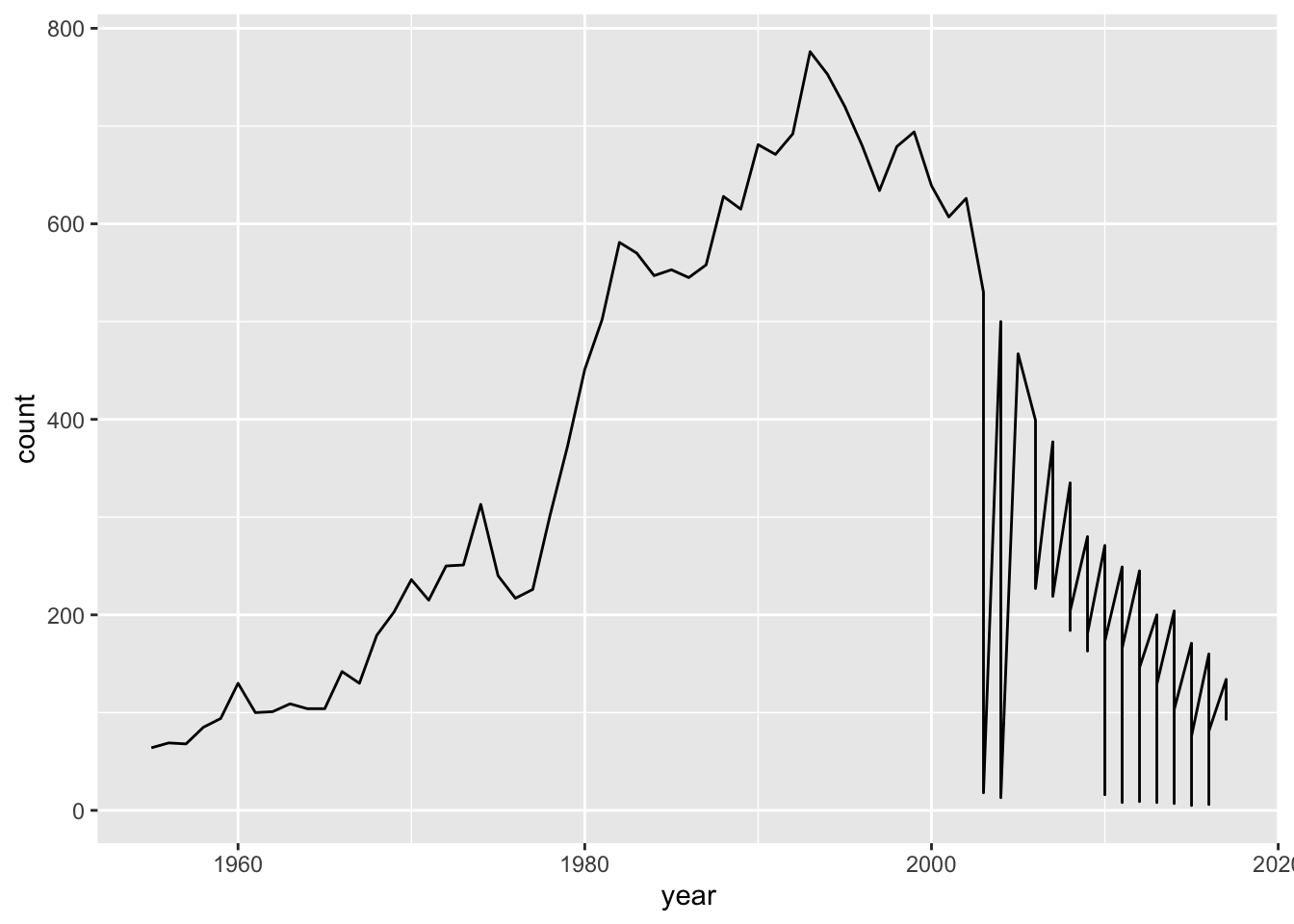
What I’m going to do it look at my name and see how often this comes up.
ozbabynames %>%
  filter(name == "Nicholas") %>%
  ggplot(aes(x = year,
             y = count)) +
  geom_line()

OK so that’s pretty good - count and year. But let’s uh, dapper this up a bit with some labs.
ozbabynames %>%
  filter(name == "Nicholas") %>%
  ggplot(aes(x = year,
             y = count)) +
  geom_line() +
  labs(x = "Year",
       y = "Count")

So that looks pretty good.
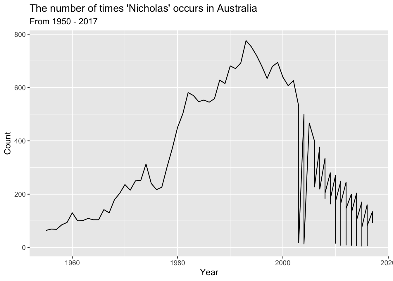
But let’s make this look a bit better - but let’s make this look really good
ozbabynames %>%
  filter(name == "Nicholas") %>%
  ggplot(aes(x = year,
             y = count)) +
  geom_line() +
  labs(x = "Year",
       y = "Count",
       title = "The number of times 'Nicholas' occurs in Australia",
       subtitle = "From 1950 - 2017")

So that’s something that is just worth knowing about, and I think it’s really neat!
The third thing: usethis::use_spell_check()
There’s a really neat feature in devtools: devtools::spell_check()
This tells me the words that it thinks has spelling mistakes - words like wikipedia, and so on. I don’t want it to pick up on all the words.
We can change that with the usethis::use_spell_check().
This adds a WORDSLIST of all of the words that are misspelt.
Now any time we run devtools::check(), it will trigger a spell check.
So this will keep me on my spelling game.
It also adds a WORDSLIST in the inst directory, which you can edit to remove the actual spelling errors.
So just, remember to use this with caution, the words list here, you will need to maintain that
